15. Architecture Reference
This section provides a deep dive into REDAC architecture, suitable for developers and experienced users who want to dig into the connectivity provided by the device. You should read the introductory section on REDAC architecture first.
15.1. REDAC Hierarchy
REDAC stands for Reconfigurable Discrete Analog Computer. This means it is constructed using discrete components, which are individual integrated circuits (ICs). These ICs house, for instance, multiple operational amplifiers (Opamps), serving as the fundamental building blocks for the electronic analog computing paradigm employed by REDAC.
The system is designed with a highly modular, hierarchical, and repetitive architecture. At each hierarchical level, components from the lower levels are arranged in a consistent, repetitive structure while remaining individually replaceable. This design achieves a balance between high regularity for efficient organization and substantial flexibility for customization. This modularity not only simplifies maintenance and scalability but also enables tailored configurations to suit specific computational needs. The following figure Fig. 15.1 provides an overview picture emphasizing on the hierarchical and modular nature of REDAC.
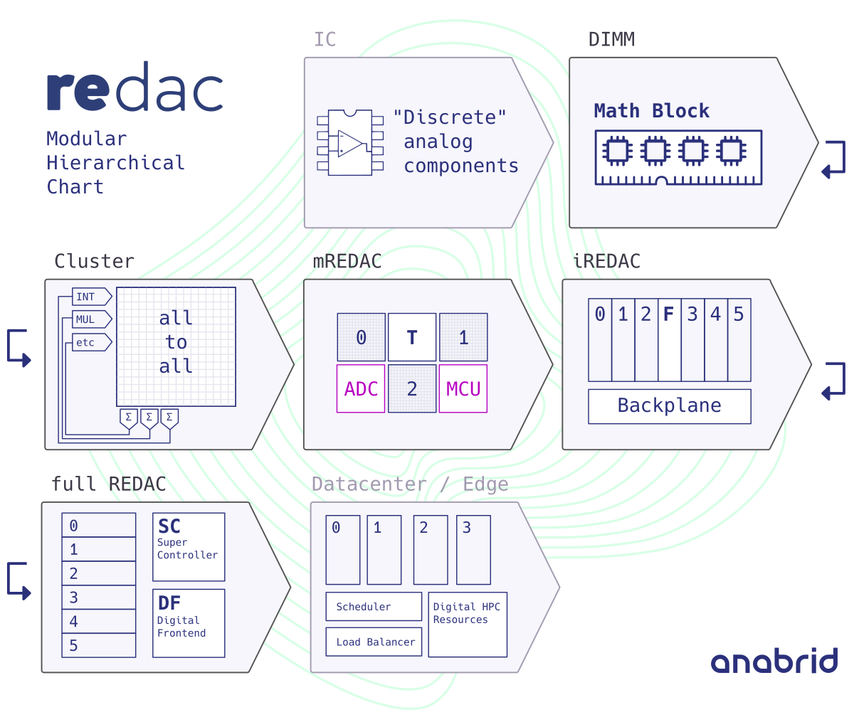
Fig. 15.1 Abstract hierarchy diagram of REDAC.
The figure introduces a lot of concepts which are presented in detail in the following sections. Despite REDAC is an analog-digital hybrid computer, the architectural description will primarily explain the analog connectivity, apart from the description of digital circuits.
15.1.1. Single cluster
A cluster is the atom of the REDAC computer. The circuits at this level are alsor refered to as macro cell in the literature. A cluster provides all-to-all connectivity between up to 16 computing elements. Coupling is implemented by switching matrices under control of the attached digital computer, basically resembling a crossbar switch.
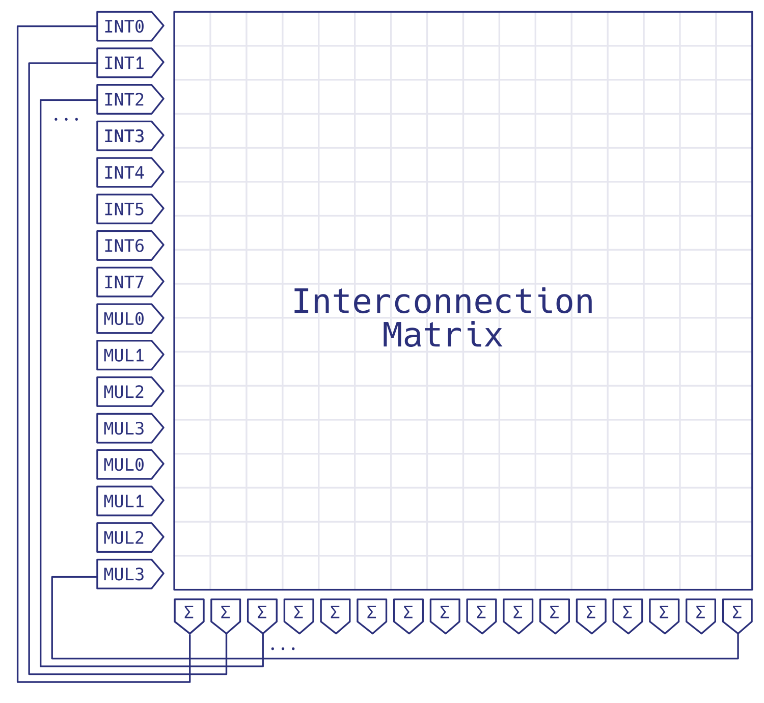
Fig. 15.2 The single cluster system reduced to its system matrix. The entries shown are for a Lorenz system.
Schematically, Figure Fig. 15.2 provides a way to visualize the interconnection matrix with real numbers representing coupling strengths. The cluster system matrix is the adjacency matrix for the interconnection graph between the computing elements. The entries are referred to as weights. As a special property, the system matrix does implicit summing which can be thought of as matrix multiplication linear algebra operations: \(C_i^\text{in} = \sum_{j=0}^{16} M_{ij} C_j^\text{out}, \quad i,j \in [0,16]\) where \(C_i^\text{in}\) is the input to the \(i\)-th computing element, \(C_i^\text{out}\) is its output, and the \(M_{ij}\) are the weights. The previous equation describes monadic computing elements with one input and one output. The integrator is the only monadic computing element in a cluster system. It computes the time integral over its time-varying input signal. REDAC also provides another kind of computing elements, which are dyadic, i.e. feature two inputs and one output: Multipliers. The multipliers implemented allow for full four-quadrant-multiplication, i.e. each of the input values can take on values within the whole machine unit interval \([-1,1]\).
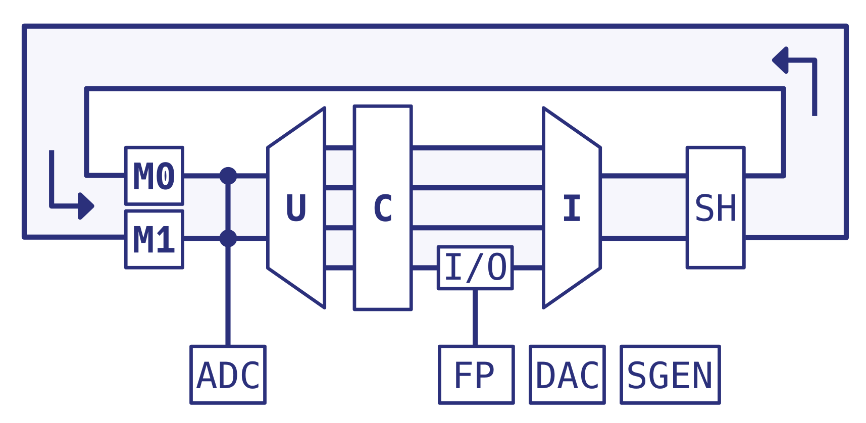
Fig. 15.3 The single cluster as a closed-loop feedback circuit (turbine diagram).
Figure Fig. 15.3 shows a more detailed block diagram of the REDAC. It shows the closed loop analog compute path. The labeled shapes in the diagram each represent a particular blocks (in bold letters, referred to as “entities” in the REDAC terminology) and auxiliary elements (in normal letters). The figure does not show any digital control/configuration signal paths. Most notably, the U-, C- and I-blocks together form the UCI matrix, which corresponds to the simplified interconnection matrix shown before in Figure Fig. 15.2. In contrast, Figure Fig. 15.3 emphasizes the internal fanout and fanin properties of the U- and I-blocks, resulting in a turbine-like appearance of this circuit representation.
The UCI matrix has 16 inputs, 16 outputs and 32 internal signal paths, each of which contains a coefficient element. These 32 paths are also called lanes and correspond to up to 32 nonzero entries in the system matrix, yielding a maximum matrix density of \(32 / 16^2 = 12.5\). This corresponds to a minimum sparsity of 87.5%.
15.1.2. mREDAC level
mREDAC stands for minimal or motherboard REDAC and is the smallest
autonomous part of the system. It contains one microcontroller (MCU)
which has an Ethernet uplink and steers all digital signals on the
motherboard. The board hosts three clusters which share a single OP/IC
line. The three clusters are interconnected by means of one T
block. This minimal self-standing analog hybrid computer is completed
with analog aquisition circuitery (eight ADC channels) as well as
digital/analog external I/O. This way, an mREDAC is basically the smallest
standalone unit of REDAC.
15.1.3. iREDAC level
iREDAC stands for intermediate or interconnecting REDAC. At this level,
seven mREDAC units are connected to a single backpanel. Interconnection
is enabled by means of several T blocks. Furthermore, several digital
busses on the back panel enable the orchestration and in particular
synchronization of the mREDACs. The iREDAC comes in a modular 19” rack-mounted
blade-style appearance where mREDACs can be conveniently accessed from the front
for maintenance purpose.
15.1.4. REDAC level
The whole REDAC system is composed by order of magnitude 10 iREDAC units. The large number of microcontrollers are steered by a single supercontroller (in short SC). This term refers both to the hardware (a single server grade computer) and a particular networking software which serves as single end point for all analog parts of REDAC. From the hardware perspective, the REDAC further contains Ethernet/IP administration (in the simplest case one switch and one router). From the software perspective, REDAC contains a managament interface ontop of the SC which does job managament, user authorization, encryption, provides API endpoints and custom software support such as compute intensive circuit transpilation. For further information on the software architecture, please refer to the Developer Manual.
15.2. Block reference
This section provides a reference of all function blocks within REDAC. Typically, a block is realized as a DIMM form factor PCB. Furthermore, typically every block is also an entity in the concept of the REDAC hybrid controller (see firmware documentation for details).
15.2.1. Cluster blocks
All blocks within a single cluster are part of the compute path and shown in figure Fig. 15.3.
M0andM1blocksM-blocks are math blocks. Each can have up to 8 analog input and 8 analog output signals. Math blocks contain various elements and allow digital configuration of these elements. In contrast to classic analog computers, there are no summers available as explicit computing elements, as summation is done implicitly in the I-block. This enhances the overall flexibility considerably. For details see Math blocks.
UblockThe output signals of these M-blocks are connected to the U-block which contains a \(16\times32\) crossbar switch. Since the output signals of the M-blocks are voltages, this crossbar switch can distribute one signal to several outputs at once. It therefore serves as a 16:32 fan-out, allowing to distribute the input signals arbitrarily on 32 internal lanes within the UCI interconnection matrix.
CblockThese \(32\) output signals (still represented by voltages) are then fed into the coefficient block. This contains \(32\) digitally controlled coefficient potentiometers with \(11\) bits resolution and an additional sign bit. Thus, the C-Block implements one coefficient per lane by means of a multiplying DAC (a certain type of digital analog converter). These coefficients allow scaling of values with factors in the interval \([-1,1]\). The output of these coefficients are now currents instead of voltages and feed the I-block.
IblockFollowing the C-block is the I-block. It, too, is a crossbar switch, this time with \(32\) inputs and \(16\) outputs. Working with currents, it is now possible to implicitly sum several inputs, thus eliminating the need for explicit summers as computing elements. The \(16\) output lines of the I-block are connected to the inputs of the computing elements contained on the M-blocks. The I-block also features a programmable gain of either factor 1 or 10, allowing for a broader dynamical range of the machine.
SHblockThis block contains 16 sample and hold elements to correct offset errors of the computing elements. It is transparent for the analog signal path and only serves for signal conditioning. It is part of the sophisticated error correction techniques of the LUCIDAC.
15.2.2. mREDAC and iREDAC level blocks
CTRLblockThis block contains the hybrid controller based on the MCU. It is responsible for setting up the computing elements, coefficient potentiometers, crossbar switches. It also takes care of the communication with the digital upstream computer (the client in a networking setting or host in a USB setting). The control block physically holds the MCU as well as eight analog to digital converters.
TblockThis block is used for interconnecting clusters. The
Tstands for tee piece but also topology or transparent. One jokes that it also stands for Tricky or T-Rex, given its highly regular yet unintiuitive way of interconnecting a large number of analog signals. TheTblock is not part of a single cluster. Each mREDAC has oneTblock and each iREDAC backplane has threeTblocks.Technically, a T-block provides 96 voltage coupled analog I/O that go to 24 analog switches. Each switch is a 1-to-3 fanout or 3-to-1 fanin, depending on the information flow in the usage mode.
15.2.3. Math blocks
Despite the implicit summing in the networking topology, all linear and nonlinear analog computation is performed on the Math blocks (M-blocks). REDAC math blocks are modular and can be exchanged, despite this requires opening the device.
A single cluster has slots for two math blocks. As of now there are two types of M-blocks available:
- Integrator Math block
MInt contains eight integrators (each with one input with implicit summing, one output). Integrators have an internal analog state (the current integration value), a digital state (IC / OP / HALT state machine), and a hybrid state (initial conditions and time scaling factor \(k_0\)).
- Multiplier Math block
MMul contains four multipliers (each with two implicit summing inputs, one output). The four remaining outputs of this block are used as identity elements. They can be used for more flexibility in the connection topology.
In normal conditions, one cluster contains eight integrators and four multipliers.
15.3. Digital Network
REDAC is truly a hybrid computer which not only features a sophisticated configurable network between the analog computing elements but also a digital network for system steering, operations and application data input/output. Compared to the analog network, the digital network is much more “off the shelf” in terms of concepts and ideas. For instance, for big throughput, REDAC internally just uses ordinary fast ethernet. See also Internal network in the operators manual for technical details about the Ethernet realization and administration.
The digital networks in REDAC fall into two conceptual groups:
Ethernet: General-purpose switching and blocking network, not supposed for low latency but highly versatile when it comes to unconventional hybrid algorithms and quick rebuilds.
Digital buses and signal lines: Real embedded and somewhat “custom” digital signaling, typically only within our own PCBs. Most of the time, unidirectionally steered by a single bus master and not time-multiplexed.
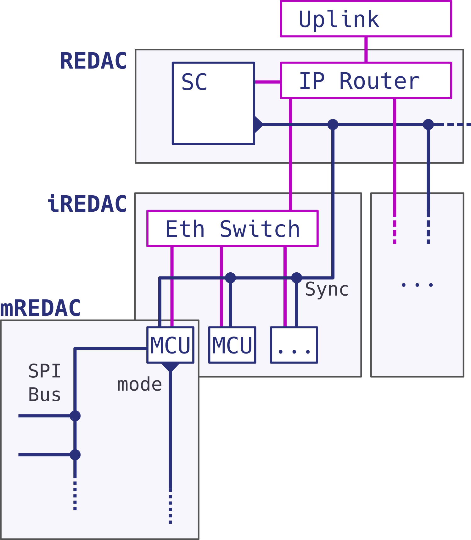
Fig. 15.4 Highlevel overview about the REDAC digital network
Figure Fig. 15.4 provides a schematic overview about the digital networking on the seperate hierarchy levels of REDAC. The conventional REDAC-internal ethernet (colored in pink) spawns between the Super Controller, Router and all microcontrollers (MCUs). On an application level, it is never used to communicate directly between the MCUs but a star toplogy is realized with the Super Controller in the center.
Within a single mREDAC, the multi-purpose digital bus is of biggest importance. It has roughly 11 address lines and roughly 5 data lines. The bidirectional bus always has the MCU as bus master and can be used in principal for any communication protocol, despite almost all chips speak (some dialect of) SPI. The bus is also extended to the iREDAC backplanes so MCUs can locate themselves and do a full “zero-knowledge” detection of adressable components at well-known address positions. Only for the first mREDAC in an iREDAC blade, the bus also reaches to programmable parts on the iREDAC level, which are for instance several T-blocks.
The sytem mode steering (IC/OP/HALT state machine) is realized in two concepts:
Within a single mREDAC, the mode is steered/distributed by the MCU with direct digital lines (GPIO outputs) at minimal latency
At iREDAC level and beyond, a custom “lowlevel subscriber scheme” is realized in a high-speed serial protocol in order to realize dynamic OP-groups, i.e. the dynamic partitioning of REDAC. This serial protocol is converted to the parallel signal distribution at MCU level. This network is sometimes refered to as sync lines since it allows multiple MCUs to synchronize their clocks over the seperate low-latency network which is superior to Ethernet.
Note that the digital network within REDAC is not supposed to be configured by neither developers nor operators. The custom digital buses have near to no configuration options anyway. For instance, typically the SPI communication parameters are dictated by the adressed chips (and can be looked up in the respective datasheets). Many parts within digital REDAC are configurable, for instance with the many EEPROMs (Entity concept) or with jumpers and dials. However, only hardware developers are supposed to change these “hard wired” settings.
15.4. Aquisition capabilities
Each iREDAC provides 8 parallel ADC channels for analog to digital signal conversion. These channels can be “hooked” onto any of the 24 computing element outputs. Each ADC can theoretically provide 1 MSample/sec, whereas the practical limit is currently about 0.5 MSample/sec. Therefore, as a rule of thumb, consider at data requesting,
sampling_rate * number_of_channels < 500_000
Where the number_of_channels is between 0 and 8 and the sampling_rate
is an integer in units samples / second. For the software interface, see
for instance the Sample rate option in pybrid.